A part of the project: Marine Analytics using Computer Vision
MOTCOM: The Multi-Object Tracking Dataset Complexity Metric
Malte Pedersen, Joakim Bruslund Haurum, Patrick Dendorfer, Thomas B. Moeslund
ECCV 2022
Multi-object tracking (MOT) covers the task of obtaining the spatio-temporal trajectories of multiple objects in a sequence of consecutive frames. Or in other words; make the computer automatically follow every object in a video. But what is it that makes MOT problems difficult to solve? Is it the total number of objects passing through the sequence (number of tracks)? Or is it the average number of objects per frame (density)? Or is it something else?
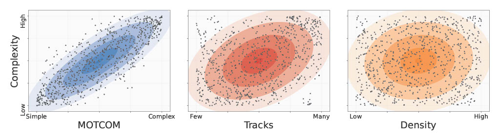
For years number of tracks and density have been the primary statistics used to describe the difficulty of MOT sequences. However, in this project we show that the number of objects (alone) is not a problem for modern trackers to handle. This is illustrated in the figure below where we have compared number of tracks and density to the complexity of the MOTSynth sequences and found no sign of correlation. The complexity is a rank-based proxy based on the HOTA performance of CenterTrack.
If one looks through the MOT literature it is often occlusion, erratic motion, and visual similarity that are either directly mentioned as obstacles or indirectly through the design of the trackers (and NOT the number of objects). Therefore, we propose the first-ever novel MOT dataset complexity metric called MOTCOM, which is based on the three aforementioned phenomena. As seen below it has a much stronger correlation with the complexity of the MOT sequences compared to tracks and density.
Challenges in MOT
There exists a range of problems in MOT sequences that are difficult to handle for trackers. We have based MOTCOM on the three aforementioned phenomena, which we deem to be the most critical, namely; occlusion, erratic motion, and visual similarity. We will describe each of the phenomena briefly in the subsections below.
Occlusion
When an object within the camera view is either partially or fully hidden we say that it is occluded. It can either be occluded by other moving objects, static objects in the scene, or simply by itself. Therefore, we say that there are three types of occlusion, which are: inter-object-occlusion, scene-occlusion, and self-occlusion.
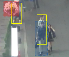
An example of inter-object-occlusion is illustrated in the image to the left by the blue bounding box where a person is walking in front of another. In the upper left corner is an example of scene-occlusion where a person is partly occluded by a scene object, in this case some flowers marked by the red bounding box.
There are cases of self-occlusion in the image, but it is non-trivial to define the level of self-occlusion and it is highly dependent on the type of object. Therefore, it is most often not taken into account in MOT systems.
Erratic Motion
In computer vision systems motion is commonly used as a term for an object’s spatial displacement between frames. This is typically because the object is moving by itself, but it can also be caused by camera motion, a combination of the two, or something else.
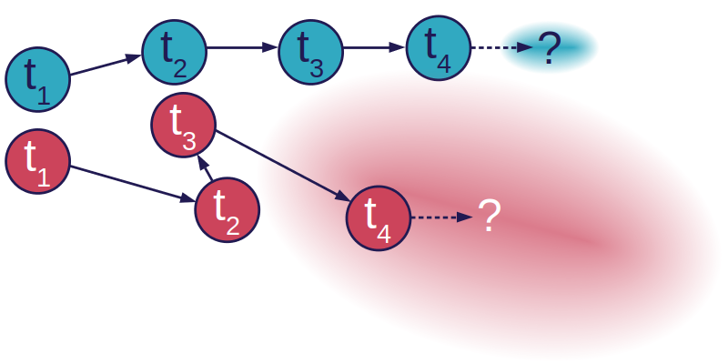
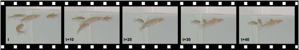
Pedestrians, cars, and bicycles often move relatively linear, which can be illustrated by the blue track in the image to the right. On the other hand, objects like prey animals (e.g., fish and flies) often move erratically and unpredictably to avoid being eaten. Such behavior is illustrated by the red track. For both tracks t1 … t4 indicates the frame number and the question mark indicates the next and unknown position of the object. Intuitively, it’s easier to predict the next state of the blue object compared to the red. This is illustrated by the two ellipsoids, which symbolize the uncertainty of the motion model.
Visual Similarity
Objects can vary widely in visual appearance depending on the type of object and type of scene. In the example below the objects looks visually similar and can be difficult to distinguish from each other. This is not necessarily a problem as long as the objects are spatially distant from each other but it becomes problematic, e.g., in the case of inter-object occlusion (as seen in the example) because re-identification methods are less certain when the object similarity increases. In other words, the spatial position of the objects is highly relevant when discussing visual similarity.
Computing MOTCOM
We propose a sub-metric for each of the aforementioned phenomena and combine them into the final MOTCOM measure. In the following subsections we describe the sub-metrics briefly, for more details please look in the paper.
OCOM: The occlusion complexity metric
The occlusion complexity metric is based on the intersection over area (IoA), which is formulated as the area of intersection over the area of the target. We only take inter-object-occlusion and scene-occlusion into account and compute OCOM as the mean level of occlusion of all the objects in the sequence. If there are ground truth annotations for the occlusion available we use them, otherwise we assume that terrestrial objects move on a ground plane. This allows us to interpret their y-values as pseudo-depth in order to decide on the ordering (to figure out who is the occluder and who is occluded). OCOM is defined in the interval [0,1] where 0 is fully visible and 1 is fully occluded. A higher value means a more difficult problem.
MCOM: The motion complexity metric
The motion complexity metric is based on core principles related to linear motion. Generally speaking, we expect that an object moves the same distance in the same direction from frame to frame. We look at the level of deviation between the expected linear path and the actual path as an expression of the complexity of the movement. This is illustrated below in figure a) where the dashed line between pt and λt+β is the expected path and the solid line between pt and pt+β is the actual path. We compute the Euclidean distance between the expected and actual position and use it to calculate the level of complexity of the motion.
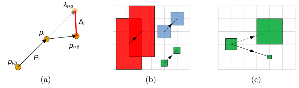
However, it is more than just the position that affects how difficult it is to track an object in motion. As illustrated in figure b) the size of the object also plays a role as it is inherently more difficult to track a small object that move a given distance compared to large object. Additionally, if an object changes in size, e.g., by moving towards or away from the camera, this also affects the complexity as the displacement is relatively less important when the size of the object increases, compared to when the size of the object decreases; this is illustrated in figure c).
Therefore, by combining these three ideas we get the final MCOM metric, which is computed as the mean size-compensated displacement across all frames and all objects at each frame. Lastly, it is weighted by a log-sigmoid function to keep the output in the range [0,1] where a higher number means a more complex problem.
VCOM: The visual complexity metric
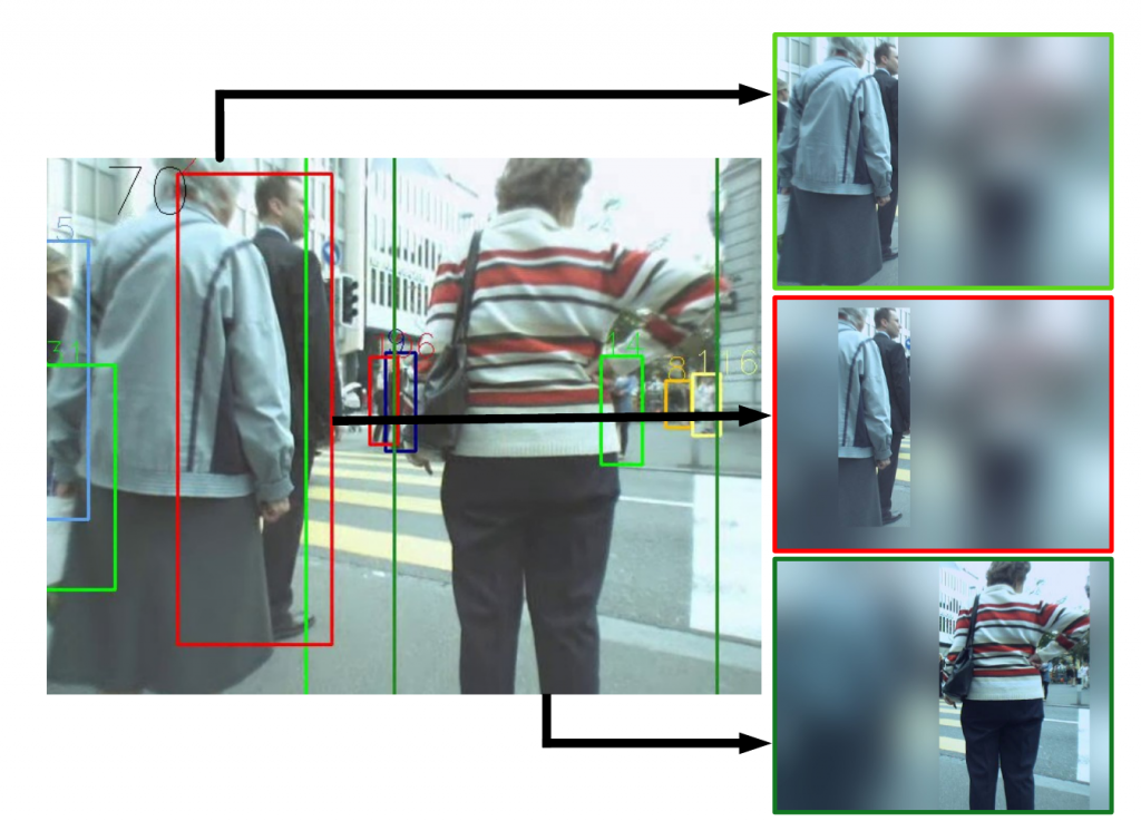
The visual complexity metric is based on three simply steps: preprocessing, feature extraction, and distance evaluation. The preprocessing step is a heavy blur using a static Gaussian kernel of size 201 with a sigma of 38. The entire image is blurred, except the object of interest as illustrated in the figure to the right. The reason for using the entire image, instead of just the bounding box, is to embed the spatial position into the feature representation and keep low level information about the surrounding.
Next, an ImageNet pretrained ResNet-18 model is used to extract features from each object-centered blurred image. And finally, the Euclidean distance is measured between the feature representation of the object of interest in frame t and the feature representations of every object in frame t+1. The distance between the feature representations is used as a measure of the similarity between the objects. If the object is visually distinct from all the other objects in the scene the closest object in frame t+1 should be the object itself.
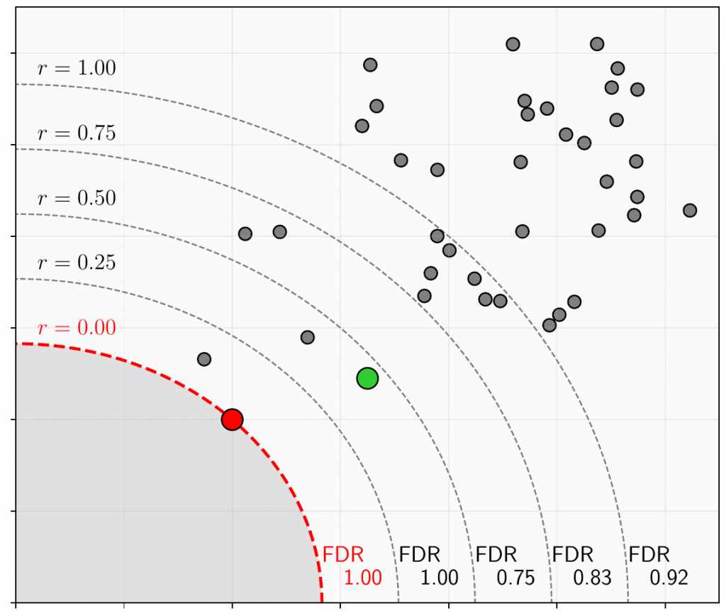
However, there may be cases where there are other objects in the proximity of the object (in the feature space) or it may even be another object that is closest. Therefore, we do not only look at the closest object, but rather the number of objects within a given distance d(r) = dNN+ dNN * r from the target object, where dNN is the distance to the nearest neighbor. This is illustrated in the figure to the right where the red dot is the target object at frame t, the green dot is the target object at frame t+1 and all the gray dots are the other objects at frame t+1.
An object within the distance boundary that shares the same identity with the target object is a true positive (TP) and the other objects are false positives (FP). This allows us to compute the false discovery rate as FDR = FP/(FP+TP) and take the mean of a range of distance ratios by changing r. The output is then a number in the range [0,1] where a higher number indicates more visually similar objects and thereby a more complex problem.
MOTCOM
Lastly, the final MOTCOM metric is computed as the arithmetic mean of the three sub-metrics:

where the weights are set to wOCOM = wMCOM = wVCOM.
Citation
@InProceedings{Pedersen_ECCV_2022,
author = {Pedersen, Malte and Haurum, Joakim Bruslund and Dendorfer, Patrick and Moeslund, Thomas B.},
title = {{MOTCOM}: The Multi-Object Tracking Dataset Complexity Metric},
booktitle = {Computer Vision -- ECCV 2022},
month = {October},
year = {2022}
}